Method at a glance
Pipeline overview
- 01Clean match history2000–2025
- 02Build team historieshome + away
- 03Roll, then shiftprevious 14 only
- 04Assemble 43 featuresform + context
- 05Cut chronologically80% / 20%
- 06Evaluate the modelsfuture matches
01 / The data
Preparing the match data
The dataset began with 12,153 Premier League matches from 1993 to 2025. Early seasons lacked the detailed match statistics needed to build consistent form features, leaving 9,329 complete matches from 2000 onward. Once every team had enough history for its rolling window, 8,827 matches remained for modeling.
What the raw data showed
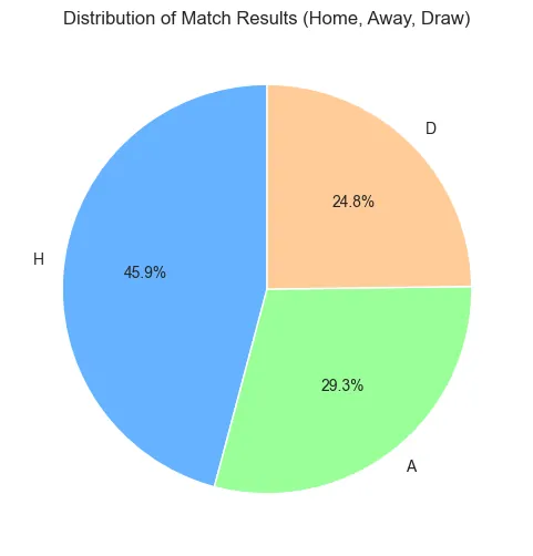
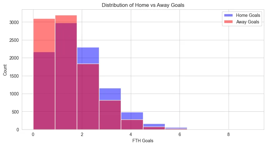
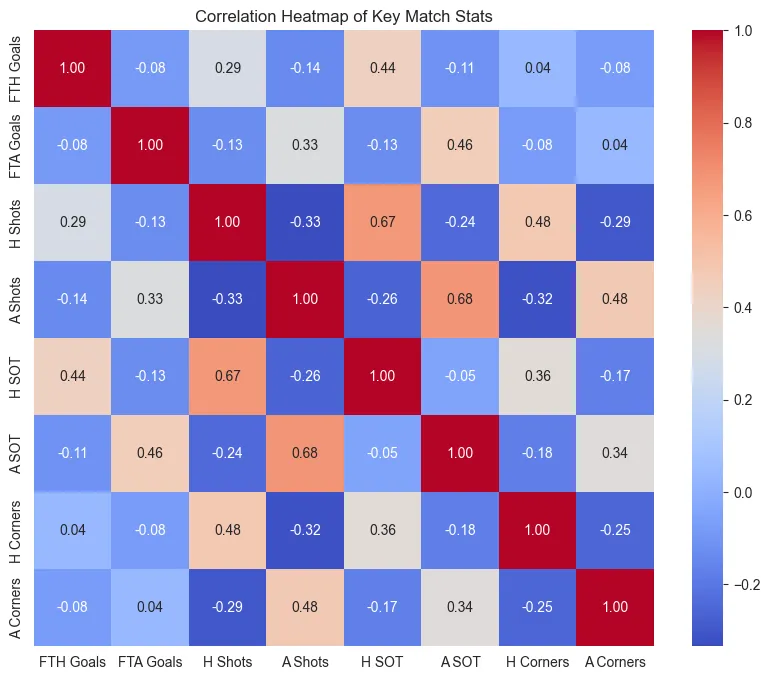
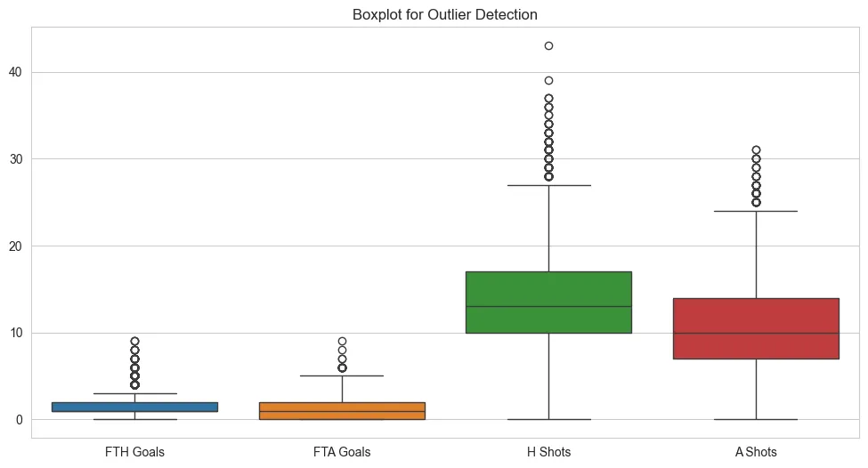
Home teams won 45.9% of the complete history, most teams scored between zero and two goals, and shots on target correlated with goals more strongly than corners. These results set the baseline and guided the feature set.
02 / Feature engineering
Rolling team form
.shift(1) move knowledge back
The fourteen green cells represent the fourteen previous matches, not forty.
.shift(1) prevents the current match from entering its own form calculation.
Rolling form
Goals, shots, corners, cards, and defensive equivalents for both teams
Matchup differences
Home attack against away defense, shot volume, and rest advantage
Closeness
Form, defense, shots, overall matchup, and season-points similarity
Season context
Home points, away points, and the difference before kickoff
Rest
Days since each team’s previous match, capped at fourteen
Time
Day of week and kickoff hour
Team identity
Home and away team encodings fitted only on training data
Season points
Season points before kickoff
Results became three, one, or zero points. Points accumulated separately inside each season, then shifted back one match before joining the model input. The model received each team’s points and the points difference, never the standings produced by the match it was predicting.
3 / 1 / 0 2Season total
cumulative 3Before kickoff
.shift(1)
Match context
Interaction and closeness features
Five interaction features measured differences such as home attack against away defense, shot volume, and rest. Five closeness features measured whether the teams arrived with similar form, defense, shots, and season points. These were designed to expose close matchups that might end level.
03 / Validation
Chronological train/test split
Team encoders were also fitted only on the training period, with an unknown-team category for promoted clubs that had not appeared before. This kept information from the test period out of both the features and the team encoding.
04 / Models
Model comparison and tuning
Across the complete dataset, always predicting a home win gives a 45.9% baseline. In the held-out future window, home wins account for 43.6% of matches. The draw-weighted run posted the highest raw accuracy by a tenth of a point but still recovered almost no draws.
05 / Feature importance
Feature importance
- 01 SeasonPointsDiff 0.0367
- 02 AT_Shots_Roll14 0.0357
- 03 HT_ShotsConceded_Roll14 0.0323
- 04 HT_Shots_Roll14 0.0314
- 05 AT_Corners_Roll14 0.0312
- 06 AT_ShotsConceded_Roll14 0.0309
- 07 HT_CornersConceded_Roll14 0.0306
- 08 AT_CornersConceded_Roll14 0.0295
- 09 AT_GoalsScored_Roll14 0.0287
- 10 HT_Corners_Roll14 0.0286
06 / Outcome recall
Draw recall remained at 2%
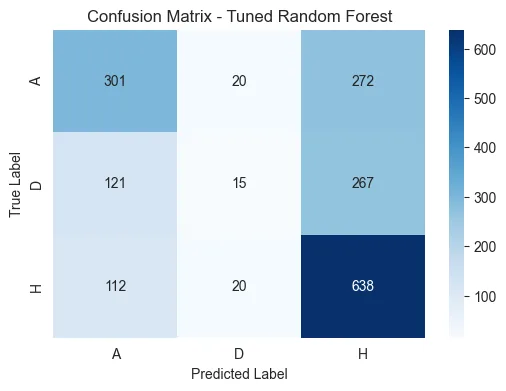
The other 388 draws were classified as a home or away win. Changing the class weights changed which matches were missed, but draw recall remained at 2%.
Limits and next steps
What the model did not have
The feature set covers team form, season points, rest, and matchup differences. It does not include match-day information.
The source data had no starting lineups, injuries, tactical changes, expected goals, betting odds, or weather. Those inputs may be useful in the close matches that the current model usually assigns to a home or away win.
A later test could add those inputs and reuse the same chronological split. It should compare probability calibration and class recall alongside overall accuracy.
Also, I implemented this in my beginnings. Don’t be too harsh, machine learning people.